Neural Architecture Search (NAS) is the process of automating the design of neural networks’ topology in order to achieve the best performance on a specific task. The goal is to design the architecture using limited resources and with minimal human intervention.
Following the work of Ren et. al, let’s discuss a general framework for NAS. At its core, NAS is a search algorithm.
-
It operates on the search space of possible network topologies, which consists of a list of predefined operations (e.g.convolutional layers, recurrent, pooling, fully connected etc.) and their connections.
-
A controller then chooses a list of possible candidate architectures from the search space.
-
The candidate architectures are trained and ranked based on their performance on the validation test.
-
The ranking is used to readjust the search and obtain new candidates.
-
The process iterates until reaching a certain condition and provides the optimal architecture.
-
The optimal architecture is evaluated on the test set.

NAS general framework
In general, the landscape of NAS algorithms is quite confusing. The most popular categorization characterizes NAS based on three major components:
a) the search space
b) the search strategy, which involves the type of controller and the evaluation of the candidates and
c) the performance evaluation technique.
You can refer to this excellent review by Esken et.al for more details. Also feel free to advice the great article by Lillian Weng as an extra resource.
However, recent approaches combine the search strategy with the evaluation step, making it hard to distinguish algorithms between them.
For that reason, we will explore NAS based solely on the search strategy. As we progress, we will examine different search spaces and evaluation techniques. Also note that many implementations experiment with different types or search strategies so the following categorization is not always strict.
Search strategy refers to the methodology used to search for the optimal architecture in the search space. We can classify NAS algorithms by their search strategy into 5 main areas:
-
Random search
-
Reinforcement learning
-
Evolutionary algorithms
-
Sequential model-based optimization
-
Gradient optimization
Random search
The most naive approach is obviously random search, which is often used as a baseline. Here a valid architecture is chosen at random with no learning involved whatsoever.
Reinforcement learning
NAS can be very elegantly formulated as an RL problem. The agent’s action is the generation of a neural architecture while the agent’s reward is the performance evaluation. The action space is of course the search space. As a result, different RL methods can be used to solve the problem.
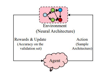
NAS with Reinforcement Learning
Early works of NAS (NAS-RL, NASNet) used a recurrent neural network (RNN) as a policy network (controller). The RNN is responsible for generating candidate architectures. The architecture is then trained and evaluated on the validation set. The parameters of the RNN controller are optimized in order to maximize the expected validation accuracy. How? Using policy gradients techniques such as REINFORCE and Proximal Policy Optimization (PPO).
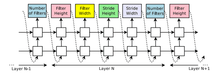
An RNN controller samples a convolutional network to predict its hyperparameters
Similarly, ENAS uses an RNN controller trained with policy gradients. Notably, it is one of the first works that effectively share parameters among architectures. The intuition is that the architectures can be viewed as part of a large graph, an approach that has been used extensively as we will see below. ENAS training is performed in two alternating steps: a) the RNN controller is trained with REINFORCE and b) the shared parameters are trained in typical gradient descent form
Another successful effort called MetaQNN uses Q Learning with an e-greedy exploration mechanism and experience replay.
Before we proceed, let’s open a parenthesis and discuss the search space,
Global search space
NAS-RL is looking for all possible combinations of operations, resulting in a huge and very expensive search space. It tried to combine the operations in order to form chain-structured (a.k.a sequential) networks. The search space is parameterized by a) the number of layers, b) the type of each operation and c) the hyperparameters of each operation (e.g kernel size, number of filters).
Later on, skip connections were also added to the mix, allowing muli-branch architectures such as ResNet or DenseNet like topologies.
Modular search space
To solve the global space problem, cell-based approaches were proposed in order to “modularize” the search space. That is, mixing different blocks of layers called modules. NASNet is the most popular algorithm in that category. NASNet learns only two kinds of modules or “cells” : a normal cell that performs feature extraction and a reduction cell that downsamples the input. The final architecture is built by stacking these cells in a predefined way.
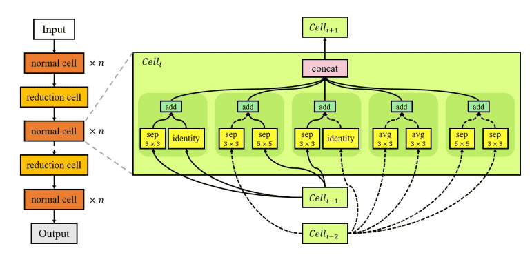
Left: An example of a search space with two cells. Right: An example of the best architecture for a normal cell as found by NAS
The cell-based approach is widely used in other works such as ENAS. But modularization via cells is not the only alternative. FPNAS emphasizes in block diversity by alternatively optimizing blocks while keeping other blocks fixed. FBNet utilizes a layer-wise search space. Each searchable layer in the network can choose a different block from the layer-wise search space.
Evolutionary algorithms
Genetic Algorithms (GA) is an alternative way to optimize the network architecture. Evolutionary algorithms start with a population of models. In each step, some models are sampled and “reproduce” to generate offsprings by applying mutations to them. Mutations can be local operations such as the addition of a layer, the modification of a hyperparameter, etc. After training, they evaluated and added back to the population. The process repeats itself until a certain condition is met.

NAS with evolutionary algorithms
GeNet proposes an encoding method to represent each architecture as a fixed-length binary string, which will be used from a standard genetic algorithm.
AmoebaNet uses the tournament selection evolutionary algorithm, or rather a modification of it called regularized evolution. The difference is that the “age” (steps of the GA) of each model is also taken into consideration by favoring the younger ones. Note that the NASNet search space is used here as well.
Sequential model-based optimization
In sequential model-based optimization, we can view NAS as a sequential process that builds more and more complex networks iteratively. A surrogate model evaluates all candidate modules (or cells) and selects some promising candidate modules. It then evaluates the performance of the generated network on a validation set and updates itself based on that performance. Through iteration, the model is gradually expanding and reaching the desired performance.
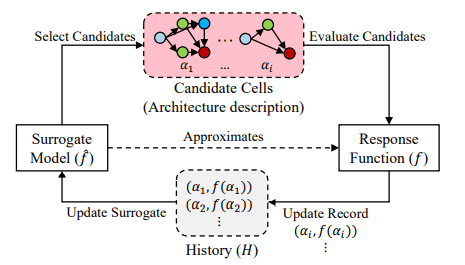
NAS with sequention model-based optimization
Progressive NAS (PNAS) starts with the NASNet search space and searches the space in a progressive order. Each cell can contain up to 5 predefined blocks. It starts by generating, training, and evaluating all possible cells with only 1 block. It then expands to cells with 2 blocks. This time though, instead of training all cells, a surrogate model (an RNN) predicts the performance of each architecture. Note that the surrogate model is trained based on the validation performance of 1-block cells. The process continues up to 5-block cells.
DPP-Net follows a very similar approach with PNAS but it also accounts for the device it’s executed on. Given the device the search is performed, constraints are set based on its memory size and similar hardware characteristics. Models that do not meet the constraints are either removed from the candidate list or optimized using Paretto optimality.
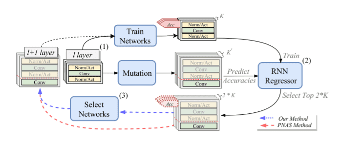
Illustration of DPP-Net’s search strategy: (1) Train and Mutation, (2) Update and Inference, and (3) Model Selection.
Gradient optimization and one-shot approaches
Gradient optimization methods use, in most cases, an one-shot model. A one-shot model, also known as supermodel ro supernet, is usually a single large network that contains all possible operations in the search space and is used to generate the weights for other candidate networks. How?
After training the model, we can use it to sample “sub-architectures’’ and compare them on the validation set. In a way, we take advantage of parameter sharing to its maximum.
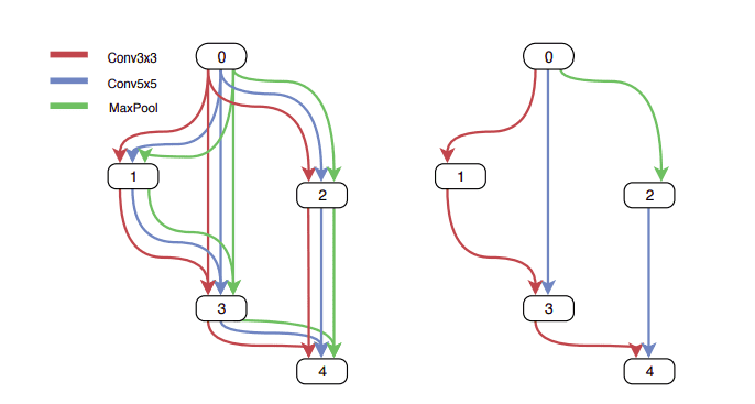
One shot architecture search
The one-shot network is usually trained with gradient descent. The question is how we can run gradient-based methods on discrete search spaces?
Continuous search space
But are we really constrained only on discrete spaces? Both global and modular search spaces assume that we have a discrete set of possible solutions. An exciting idea is to transform the space into a continuous and differentiable form.
In this direction, DARTS relaxes the NASNet cell-based space in a continuous way by representing each cell as a node in a Directed Acyclic Graph (DAG). Every DAG is formed as a sequential connection of N nodes and has two input nodes and one output node. The relaxation is performed by formulating the discrete choice of operations as a softmax; a continuous choice of probabilities.
DARTS treats NAS as a bi-level optimization problem because it jointly trains the architecture parameters and network weights with gradient descent.
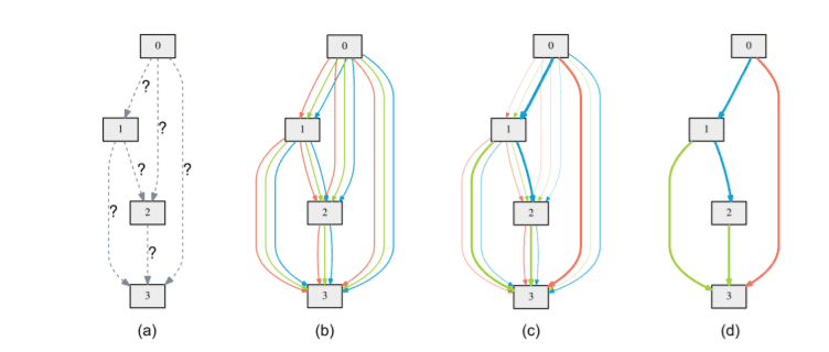
Illustration of DARTS: (a) Operations on the edges are initially unknown. (b) Continuous relaxation of the search space. (c) Joint optimization of the mixing probabilities and the network weights (d) Inducing the final architecture
In a very similar way, Stochastic NAS (SNAS) search space is a set of one-hot random variables from a fully factorizable joint distribution. This search space is made differentiable by relaxing the architecture distribution with concrete distribution, thus enabling the use of gradient optimization.
NAO, on the other hand, maps the discrete search space to continuously embedded encoding. That way, they can obtain the optimal embedded encoding using gradient optimization. A decoder is then used to discretize the optimal continuous representation into the final architecture.
One shot approaches
Both DARTS and NAO fall into one-shot approaches because they use a supermodel to deduct the optimal architectures. Let’s explore some other ones.
SMASH trains an auxiliary model called HyperNet instead of training all possible candidates, reducing the search space even further. The HyperNet is used to generate the weights for other candidate networks. How?
At each training step, they choose a random architecture and feed a description of it (in the form of a one-hot tensor) to the HyperNet in order to generate its weights. After training the entire system, they compare a bunch of sampled architectures with their generated weights on the validation set. The “best” one is then trained normally.
ProxylessNAS proposes a path-level pruning perspective. Its other major contribution is this idea of binarizing the architecture parameters in order to have only one active path at a time. The probability that a path will be pruned or not (architecture parameters) are learned jointly with the weights parameters
So starting with an over-parameterized network with all candidate paths, the training executes the two following steps alternatively:
-
The training of weight parameters is performed by sampling only one path at a time and training it using gradient descent. Note that the remaining architecture parameters are frozen during this step.
-
The architecture parameters are trained using BinaryConnect, while the weights parameters are frozen.
Once the training of architecture parameters is finished, they derive the final architecture by pruning redundant paths.

Learning process of both weight parameters and architecture parameters on the Proxyless NAS approach
Single Path One-Shot (SPOS) constructs a simplified supermodel, where all architectures are single paths. They also eliminate the need for the joint distribution of architecture parameters and weights we previously saw, by decoupling the supernet training and architecture search in two distinct steps.
The supernet optimization is done by simply sampling paths in a uniform manner while the actual NAS is performed with an evolutionary algorithm.
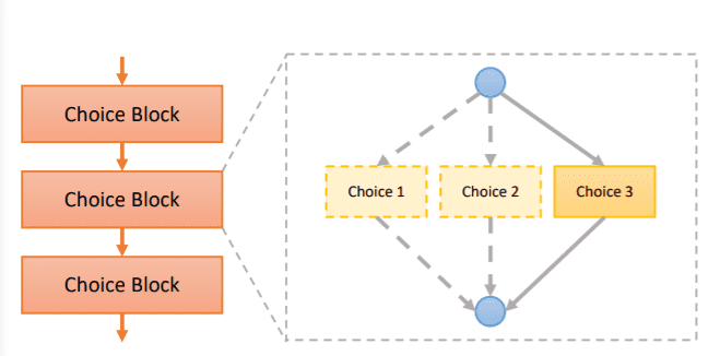
Choice blocks for a single path supernet
AlphaNet builds on top of previous works (Liu et al), which used in-place knowledge distillation (KD) to handle NAS. By distilling the knowledge of the supernet (teacher), they can greatly improve the performance of sub-networks. Standard KD is usually formulated with KL divergence which quantifies the difference between teacher and students. AlphaNet takes it a step further and applies alpha-divergence to the problem, improving the training of the supernet. At the time of writing this article, AlphaNet achieves top-1 accuracy on the ImageNet dataset according to benchmarks shown in paperswithcode.com.
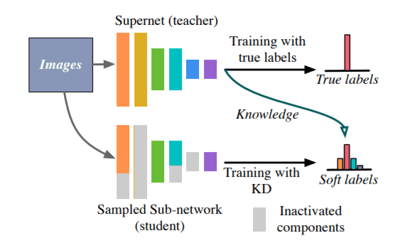
An illustration of training a supernet with knowledge distillation
Another top-1 model is BossNAS. BossNAS (Block-wisely Self-supervised Neural Architecture Search) adopts a novel self-supervised representation learning scheme called ensemble bootstrapping. The authors first factorize the search space into blocks. It is worth mentioning that the original work focuses only on vision models and uses a combination of CNN and transformer blocks.
The supernet is also trained with self-supervision, in a fashion similar to BYOL. Two siamese supernetworks are learning the representation using a pair of augmented views of the same image and minimizing the distance between their outputs. The subnetworks are trained to predict the probability ensemble of all the sampled ones in the supernet. The probability ensemble is used as the evaluation metric of the sampled models.
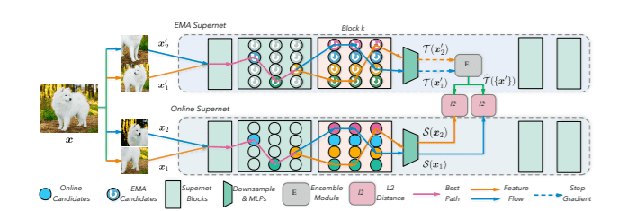
Illustration of two Siamese supernets training
Neural Architecture Transfer
The authors of NAT (Neural Architecture Transfer) had this idea of using transfer learning in the context of NAS by transferring an existing supernet into a task-specific supernet. At the same time, they can also search for architectures that better solve the multiple objectives of interests. Thus, combining transfer learning with the search process.
Multi-objective refers to the presence of multiple conflicting objectives. In multi-objective problems, the algorithms should account for all objectives by offering the best trade-offs between them. In the context of NAS, examples of objectives include inference time restrictions, memory capacity, size of the final model etc. Multi-objective NAS is a research area that is evolving rapidly.
NAT is divided into three components: a) an accuracy predictor b) an evolutionary search process and c) a supernet. The whole process goes as follows:
-
Starting from a list of trained supernets, they uniformly sample a set of them.
-
The performance of the supernets is evaluated.
-
The accuracy predictor is then constructed with the goal to drive the search taking into account the multiple objectives.
-
The evolutionary search proposes a set of promising architectures
-
The architectures are back to the original list of supernets and the process iterates until satisfying a terminal condition.
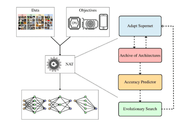
Illustration of the Neural Architecture Transfer process
Implementation with neural network intelligence (nni)
For better understanding, we will also present an example implementation of NAS using the neural network intelligence (nni) package by Microsoft. There are other AutoML libraries out there that support NAS such as AutoKeras, Auto-Pytorch, AutoGluon but nni is by far the most complete and well maintained. nni supports a variety of methods. Examples include: PPO-based methods, AmoebaNet, ENAS, DARTS, ProxylessNAS, FBNet, SPOS and more.
Since one-shot models outperform other techniques consistently and it’s the main research direction at the moment, we will showcase how to execute them with nni. The simplest approach is the DARTS algorithm.
The showcase code can be found in this colab notebook. Note that it’s heavily inspired by the official examples and tutorials of the nni library.
DARTS uses a supergraph as its search space. Each cell is regarded as a DAG and they are combined into a multi-path supermodel. To declare a cell, nni provides the LayerChoice which accepts multiple standard Pytorch modules (convolutional, pooling etc). That way, it defines multiple paths inside the supermodel. After training, only one path will be chosen to form the optimal architecture.
self.conv1 = nn.LayerChoice([nn.Conv2d(3, 6, 3, padding=1), nn.Conv2d(3, 6, 5, padding=2)])
Another option is to use the InputChoice module, which is primarily used to explore different connections. In our example, we will use skip connections. The end architecture will either keep the skip connection or not.
self.skipconnect = nn.InputChoice(n_candidates=2)
x1 = self.skipconnect([x1, x1+x0])
The supergraph can be defined as a typical Pytorch model, but instead of using the original Pytorch package, we need to use the one provided by nni. An example can be found below:
import torch.nn.functional as F
import nni.retiarii.nn.pytorch as nn
class Net(nn.Module):
def __init__(self):
super().__init__()
self.conv1 = nn.LayerChoice([nn.Conv2d(3, 6, 3, padding=1), nn.Conv2d(3, 6, 5, padding=2)])
self.pool = nn.MaxPool2d(2, 2)
self.conv2 = nn.LayerChoice([nn.Conv2d(6, 16, 3, padding=1), nn.Conv2d(6, 16, 5, padding=2)])
self.conv3 = nn.Conv2d(16, 16, 1)
self.skipconnect = nn.InputChoice(n_candidates=2)
self.bn = nn.BatchNorm2d(16)
self.gap = nn.AdaptiveAvgPool2d(4)
self.fc1 = nn.Linear(16 * 4 * 4, 120)
self.fc2 = nn.Linear(120, 84)
self.fc3 = nn.Linear(84, 10)
def forward(self, x):
bs = x.size(0)
x = self.pool(F.relu(self.conv1(x)))
x0 = F.relu(self.conv2(x))
x1 = F.relu(self.conv3(x0))
x1 = self.skipconnect([x1, x1+x0])
x = self.pool(self.bn(x1))
x = self.gap(x).view(bs, -1)
x = F.relu(self.fc1(x))
x = F.relu(self.fc2(x))
x = self.fc3(x)
return x
model = Net()
Once we declare the supergraph, we can define the NAS training using the DartsTrainer class. DARTS requires a metric to evaluate each candidate architecture as well as typical training arguments ( optimizer, loss, number of epochs etc). In a way, it’s similar to training a standard deep network.
import torch
from nni.retiarii.oneshot.pytorch import DartsTrainer
def accuracy(output, target):
batch_size = target.size(0)
_, predicted = torch.max(output.data, 1)
return {"acc1": (predicted == target).sum().item() / batch_size}
criterion = torch.nn.CrossEntropyLoss()
optimizer = torch.optim.SGD(model.parameters(), lr=0.001, momentum=0.9)
trainer = DartsTrainer(
model=model,
loss=criterion,
metrics=lambda output, target: accuracy(output, target),
optimizer=optimizer,
num_epochs=1,
dataset=train_dataset,
batch_size=64,
log_frequency=10
)
trainer.fit()
After training, we can obtain the optimal architecture. The nni API will provide it in the form of “mutations”. The mutations are showing which cell topology DARTS decided to keep. For each cell, we will get a mutation showing the best topology.
In our case, the first conv layer will be formed by the fist declared block (nn.Conv2d(3, 6, 3, padding=1)) while the second by the second (nn.Conv2d(6, 16, 5, padding=2)). Skip connections have been found to also provide better results, so we are keeping them (mutation_3).
print('Final architecture:', trainer**.**export())
nni is much richer than we are able to show in a single article, so we highly recommend playing around with it.
Note that the first part of the Machine Learning Modeling Pipelines in Production course by Robert Crowe is solely dedicated to NAS, so make sure to check it out.
Conclusion
NAS research is still in its infancy in my personal opinion. Benchmarking is also not a trivial endeavor. At the moment, we have some standard benchmarks such as ImageNet, NAS-Bench0201, CIFAR10, but more work is definitely needed in this direction. Finally open source libraries, with the exception of nni, are barely touching NAS as a problem.
I hope that this review serves as an introduction and will motivate more practitioners to pursue NAS as their research topic. For any questions, possible mistakes or additions, feel free to ping us on our Discord server.
Cite as
@article{karagiannakos2022nas,
title = "Neural Architecture Search (NAS): basic principles and different approaches",
author = "Karagiannakos, Sergios",
journal = "https://theaisummer.com/",
year = "2021",
howpublished = {https://theaisummer.com/neural-architecture-search/},
}
References
* Disclosure: Please note that some of the links above might be affiliate links, and at no additional cost to you, we will earn a commission if you decide to make a purchase after clicking through.
