This follow-up blog post reviews alternative classifier-free guidance (CFG) approaches to a diffusion model trained without conditioning dropout. In such cases, CFG cannot be applied. So, what do we do? Or how do we apply CFG in purely unconditional generative setups?
Recent works reveal that the (jointly trained) unconditional “model” can be substituted with various alternatives, such as an impaired/inferior model. The inferior network can be conditional or unconditional and requires, by design, some sort of bottleneck compared to the conditional model. We will refer to the positive and negative models to avoid confusion between the conditional and unconditional models, as in plain CFG. Visit our previous articles on diffusion models or CFG to grasp the fundamental concepts first.
Positive and negative notation
CFG requires a) an external condition (text or class label) and b) training both with and without the condition. The latter refers to randomly dropping the condition, typically 10-20% of the time. Separate training of models can also be conducted, but in both cases, it’s a limitation. This was a known limitation of CFG, and it was one of the reasons for its initial rejection:
“From the AC’s perspective, the practical significance could be enhanced if the authors can generalize their technique beyond assisting conditional diffusion models.”
From now on, we will refer to the conditional and unconditional models in CFG as positive and negative models due to their sign in the CFG equation.
This generalizes the framework beyond the use of a condition, allowing for arbitrary models to be combined. We use the “negative” model instead of the unconditional one for extrapolation. Typically, the positive model is a regular diffusion model, and the negative model is a modified version of the positive model. We find this generalized framework of positive and negative terms in the CFG equation helpful and use it in this article.
The generalized formulation of CFG was first presented by Hong et al. 2023. Then, the big question boils down to: what should we use instead of the negative term instead of the unconditional model?
Self-Attention Guidance (SAG)
TL;DR: The negative model is the same as the positive model, but its predictions are modified via. The main idea is to replace the unconditional model with a conditional model with blurred patches. Patches with high activation based on the self-attention map are blurred (adversarial blurring).
Hong et al. try to develop a method, namely self-attention guidance (SAG), that
-
works out of the box for both conditional and unconditional models
-
aims to apply CFG-like guidance on any single diffusion model (unconditional or conditional) with a noised image as an input.
-
Manipulates the input image (we will see how) to generate the negative term.
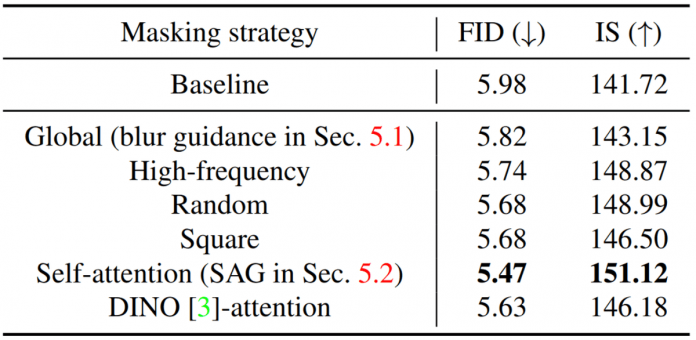
The authors of SAG try to develop ideas to derive a useful signal that can act as a negative term on the CFG equation. In their terms, they ablate with various “masking strategies” in image space and measure the impact on FID.
To the best of our understanding, “baseline” in the table below refers to the conditional ADM diffusion model on ImageNet at 128×128 resolution. Based on the ablation study below, one can deduct the following:

Ablation study of the masking strategy (). The results are from ADM trained on ImageNet . The table is taken from , licensed under CC BY 4.0. No changes were made.
-
Gaussian blur guidance (“global”) performs smoothing via local intensity weighted averaging as a negative term at each step. Blurring reduces the local details (high frequency) within the input signals.
-
High frequency refers to applying a high-frequency mask using FFT on the denoise image. If I understand correctly, the high-frequency mask would keep the high frequencies and attenuate or remove the low frequencies from the signal.
-
Random and square reset the value pixels.
-
SAG and DINO use attention maps and apply Gaussian smoothing (blur) only in high-activation patches. The authors show an overlap of attention maps generated from a diffusion model with high-frequency signals in the image. DINO is a pre-trained self-supervised vision transformer that has never seen noisy images.
It is crucial that the attention map needs to be manually picked (there are L x H attention maps for L layers and H heads) and upscaled to the image size i.e. from 16×16 to 224×224.
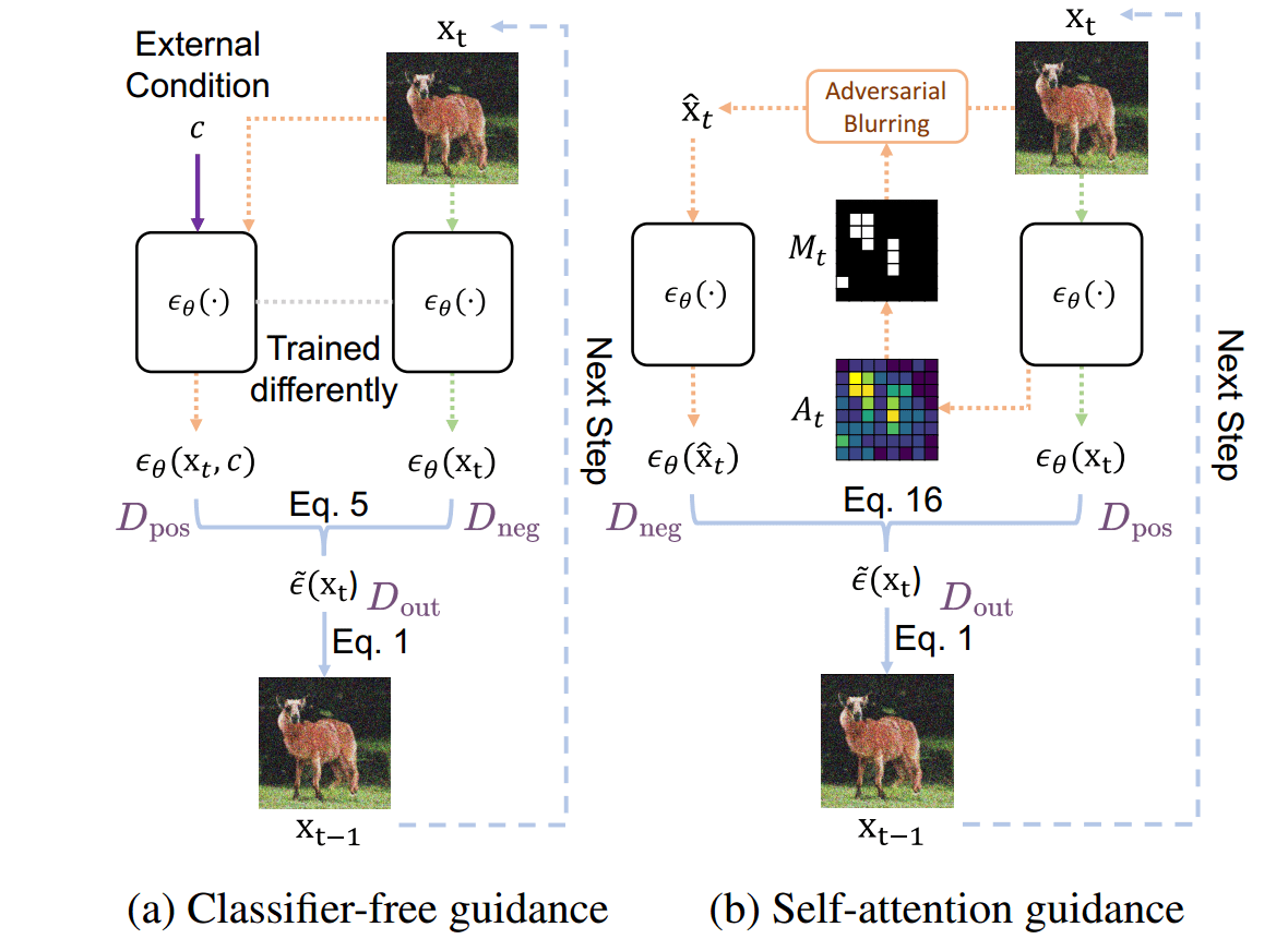
Compared to CFG, which uses external class information, SAG extracts the internal information with self-attention to guide the models, making it training- and condition-free. The figure is adapted from with minor annotations highlighted in light purple, licensed under CC BY 4.0.
Their results point to the fact that subtracting high-frequency information is more beneficial, similar to other studies. In the above figure, I have highlighted in purple which term is positive and which is negative to avoid confusion.
Instead of blurring the whole image (high-frequency filtering), SAG blurs the image patches with the highest attention activations. Read our previous blog post for more info on how self-attention works in diffusion models .
The improvement in FID compared to the baseline is less than 10 %, yet the presented images look better. However, due to aggressive perturbation applied directly to the model’s input, SAG has recently shown a tendency to produce out-of-distribution (OOD) samples and high hyperparameter sensitivity .
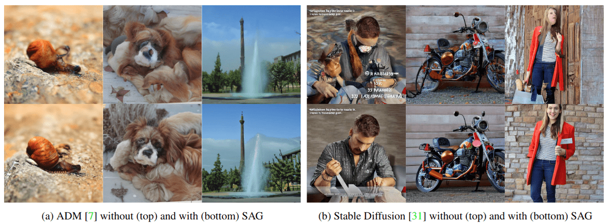
Cheery picked qualitative comparisons between unguided (top) and self-attention-guided (bottom) samples. Unlike classifier
guidance or classifier-free guidance (CFG)], self-attention guidance (SAG) does not necessarily require an external condition, e.g., a class label or text prompt, nor additional training: (a) unconditional ADM and (b) Stable Diffusion with an empty prompt. Source
The concern when doing guidance with impaired models boils down to increasing quality without introducing new artifacts. This method is the first one that indicated this direction to the community, so it is worth some credit!
Attention-based self-guidance: perturbed self-attention (PAG)
Narrative: This work employs a conceptually similar approach to SAG, aiming to derive a training-free negative term from the same model. However, instead of attention-based adversarial image blurring, it directly impairs the attention module in the UNet, breaking the samples’ semantic structures. The resulting difference in CFG between positive and negative terms is intended to repair the semantic coherence of the final generated sample.
TL;DR: The negative term is formed by substituting a few self-attention matrices in the UNet’s encoder with an identity matrix. Works for conditional and unconditional models as positives.
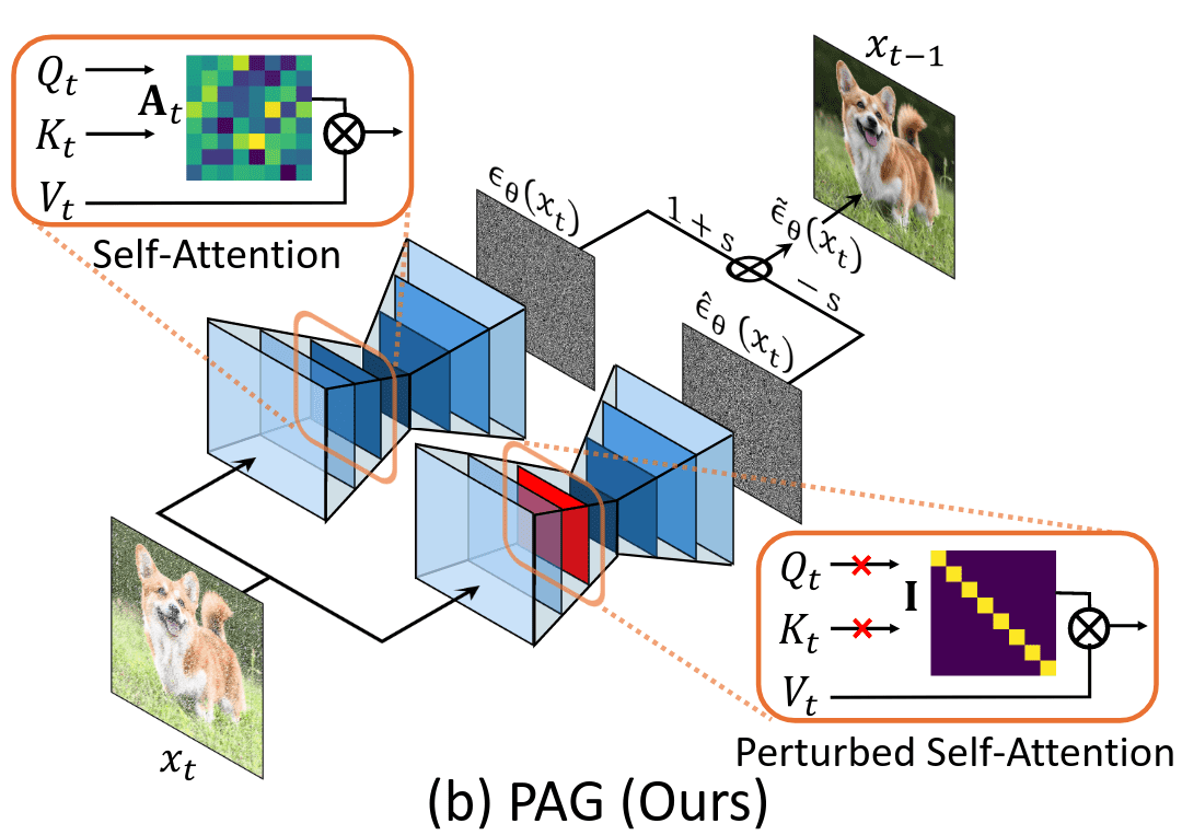
PAG replaces the self-attention map with an identity matrix for the negative model. Source
Ahn et al. attempt to derive the guidance signal from a single network. To this end, they define various perturbations denoted as that can be applied in conditional and unconditional models, similar to the “masking strategy” ablation study of SAG . This is the same as the negative term we have previously defined.
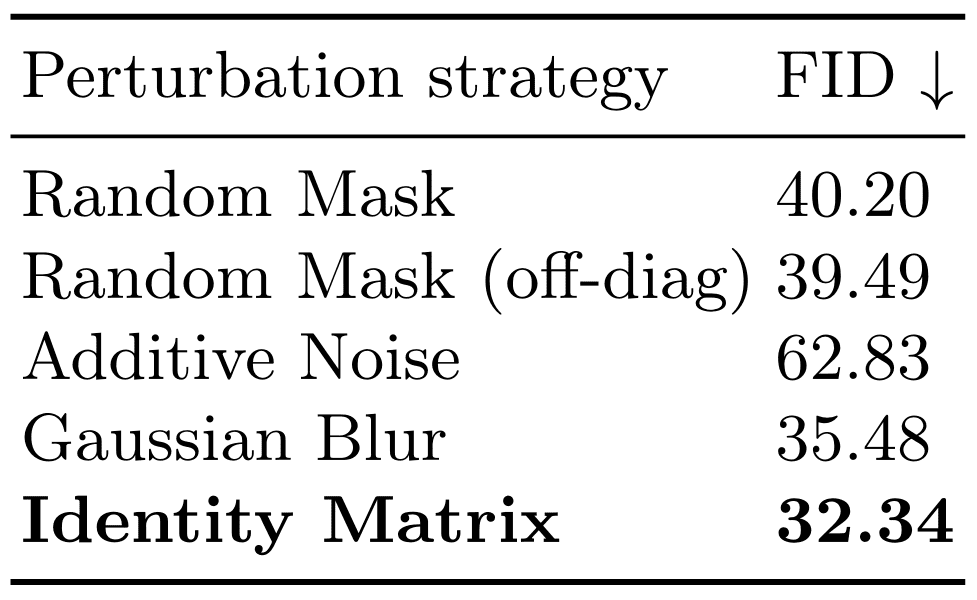
Ablation study on different perturbations on the self-attention mask for . The unconditional ADM model is used with 5K images on ImageNet 256×256. The same guidance scale of is used. Source
The key concept is that the negative/perturbed term has an undesirable property we wish to move away from, based on the forward pass of an already trained denoiser . A perturbation can be applied to the input , such as blurring or high pass frequency filter, on the internal representation of the diffusion model, or both. To design the perturbation strategy, Ahn et al. focus on the attention mechanism of denoising U-Nets. Similar to cross-attention in the previous studies (such as Hertz et al. 2022), they argue that self-attention matrix contains structural information while related to the “appearance”
This simple approach replaces the selected self-attention map with an identity matrix .
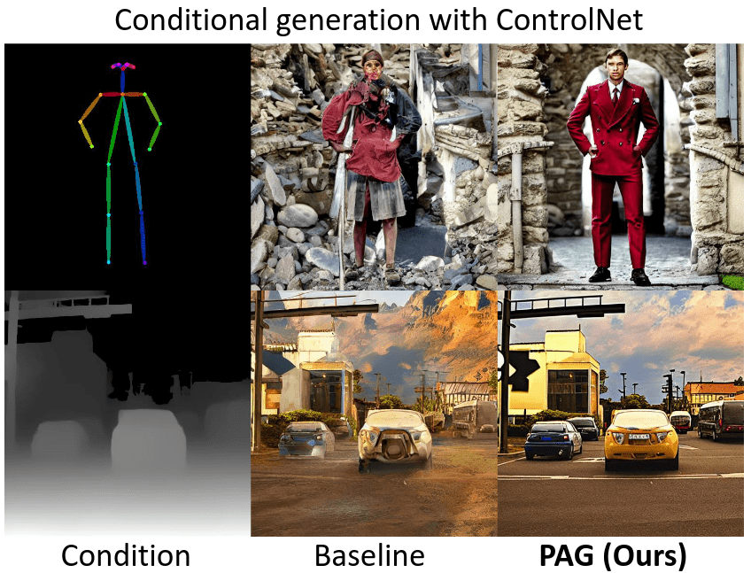
Qualitative comparisons between unguided (baseline) and perturbed-
attention-guided (PAG) diffusion samples. Source
However, both methods (SAG and PAG) remain architecture-dependent: which layers of the Unet am I supposed to select? What If my Unet is larger or smaller than the one used in the paper? What if I don’t have a Unet model?
Autoguidance: Guiding a Diffusion Model with a Bad Version of Itself
Narrative: This work distills the idea of creating a negative model from an impaired positive one into a simpler form. The core intuition is that the negative model should make errors similar to the positive one but stronger.
TL;DR: Create the negative term in CFG with a “weak” model, achieved by i) training the network less (using an earlier checkpoint), ii) using a network of smaller learning capacity (fewer parameters). Combining the two achieves state-of-the-art generative performance in class-conditional models on ImageNet.
The vanilla version of CFG is only applicable to conditional generation. Since the denoiser is trained with two objectives (task discrepancy), the sampling trajectory of CFG can overshoot the conditional distribution. Finally, the prompt alignment is controlled by the guidance scale but harms visual metrics such as FID. Karras et al. demonstrate how to disentangle the above effects and control them in isolation. In the vanilla CFG setup, the denoiser has a more difficult task than . tries to fit and generate all classes at once, whereas can focus on a single condition.
Autoguidance refers to leveraging an inferior version of the denoiser (), as the negative/guiding model . can be obtained by simply limiting model capacity and/or training time. As such, autoguidance enables CFG-like guidance for unconditional image synthesis.
They find that the positive model can be bottlenecked by reducing the number of parameters or training iterations. In this way, the positive and negative are both conditional or, as the authors describe it:
“Our method does not suffer from the task discrepancy problem because we use an inferior version of the main model itself as the guiding model, with unchanged conditioning.”
Intuition. The intuition behind autoguidance is that the weak model is prone to make similar yet stronger errors, likely in the same regions. Autoguidance seeks to boost the difference of these errors via step-wise extrapolation. The worse the negative term, the more intensified the difference. Lowering the model’s capacity by lowering the number of parameters and using a smaller training budget achieves the desired property.
In practice, a well-tuned combination of smaller size models, e.g. between 30 to 50 % of the parameters, and a shorter training schedule () was experimentally found to work well on the ImageNet scale.
The models’ EMA is a 3rd nuanced hyperparameter pair influencing the balance between positive and negative terms during sampling. To decide upon the best EMA hyperparameter (), Karras et al. store multiple pre-averaged models during training. The saved pre-averaged model weights from different training iterations can be linearly combined after training: . This decouples the hyperparameter tuning from training, and one can perform a grid search during sampling. This, however, overcomplicates the sampling process!
In the table below, the authors emphasize that
-
using a smaller EMA value for the main model (positive) is beneficial in practice.
-
using an earlier checkpoint is more impactful than using a model of inferior capacity.
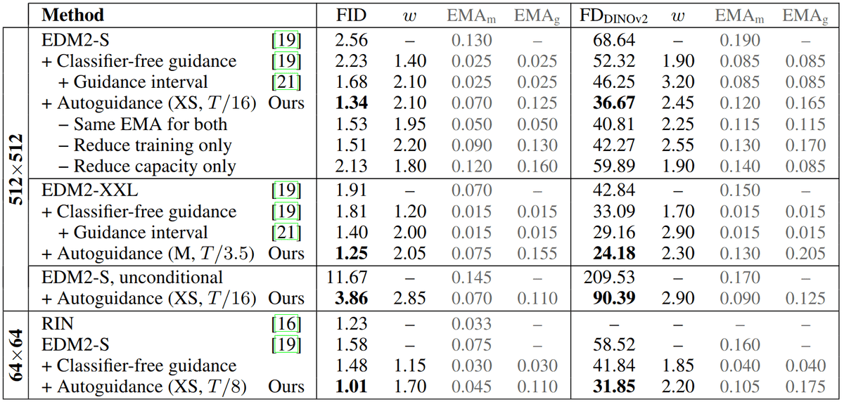
Results on ImageNet-512 and ImageNet-64. The parameters of auto-guidance refer to the capacity and amount of training received by the guiding model. The latter is given relative to the number of training images shown to the main model (T). The columns and indicate the length parameter of the post-hoc EMA technique for the main and guiding model, respectively. The table snapshot is taken from . No changes were made.
Below, you can find the curves that show the individual factor sensitivities:

Sensitivity w.r.t. autoguidance parameters, using EDM2-S on ImageNet-512. The shaded
regions indicate the min/max FID over 3 evaluations. (a) Sweep over guidance weight w while
keeping all other parameters unchanged. The curves correspond to how much the guiding model was trained relative to the number of images shown to the main model. (b) Sweep over guidance weight for different guiding model capacities. (c) Sweep over the two EMA length parameters for our best
configuration, denoted with ⋆ in (a) and (b). Source
The price you pay to get such good numbers is that this is not a training-free approach if you want to train a smaller model and the vast hyperparameter search during inference (model size, which checkpoint, EMA positive, EMA negative). Finally, if you train your do not your own models, you will only have a single publicly available checkpoint, rendering the method impractical for such cases.
No Training, No Problem: Rethinking Classifier-Free Guidance for Diffusion Models
ICG: Another training-free solution is independent condition guidance (ICG) : sample a random condition as negative instead of unconditional. The purpose of this approach is to provide a training-free alternative for conditional models that have not been trained with conditional dropout. Below are some cherry-picked results from the paper :
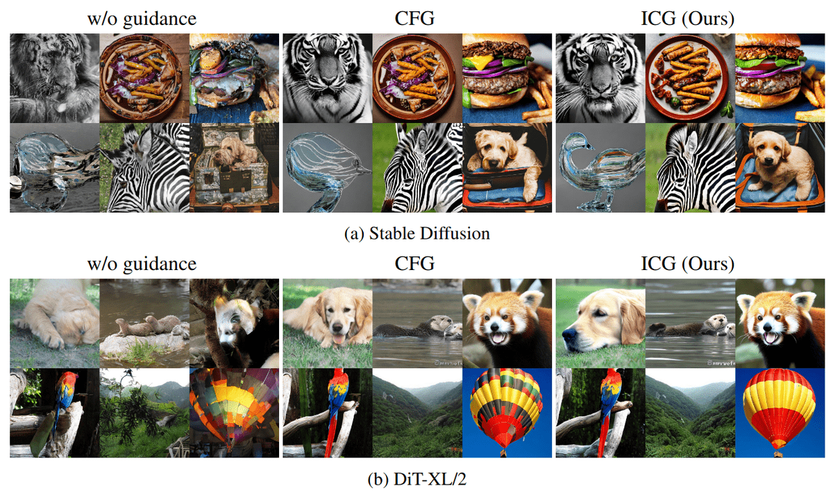
Comparison between CFG and ICG for (a) Stable Diffusion and (b) DiT-XL. Both CFG and ICG improve the image quality of the baseline. Source
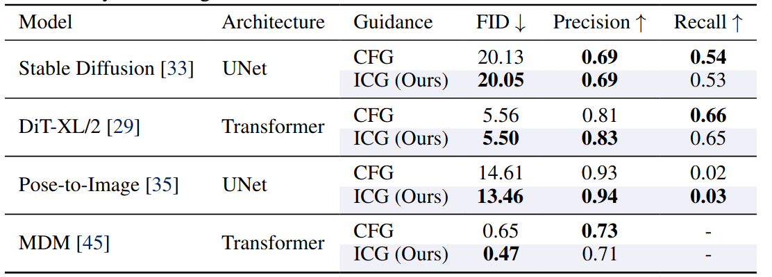
Quantitative comparison between CFG and ICG. ICG is able to achieve similar metrics to the standard CFG by extracting the unconditional score from the conditional model itself. Source
Nonetheless, this solely applies to conditional models. It is worth mentioning that the same authors propose a similar variant for unconditional models that applied a hacky perturbation on the timestep embedding of the unconditional model.
Self-improving Diffusion Models with Synthetic Data
Another fantastic idea is to re-train your (trained) diffusion model with a re-training budget B with its own synthetic samples to create the impaired model. Then, the sample of the impaired model is used as a negative in a CFG-like fashion.
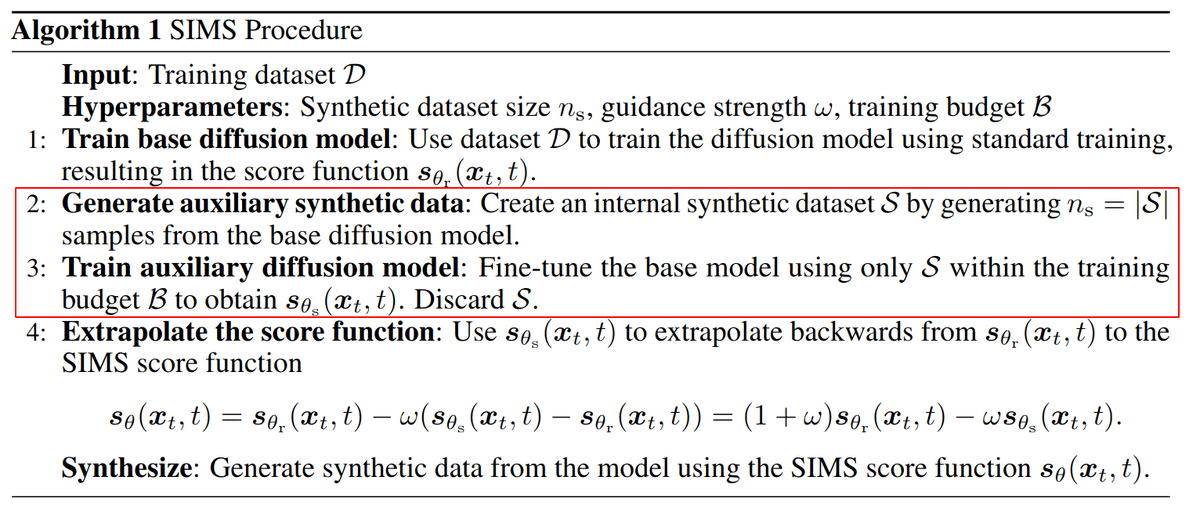
Algorithm description of SIMS: Self-improving Diffusion Models with Synthetic Data. Source
Now, one must decide on the hyperparameters: synthetic dataset size and re-training budget.
The authors chose the synthetic dataset size to roughly match the real dataset size.
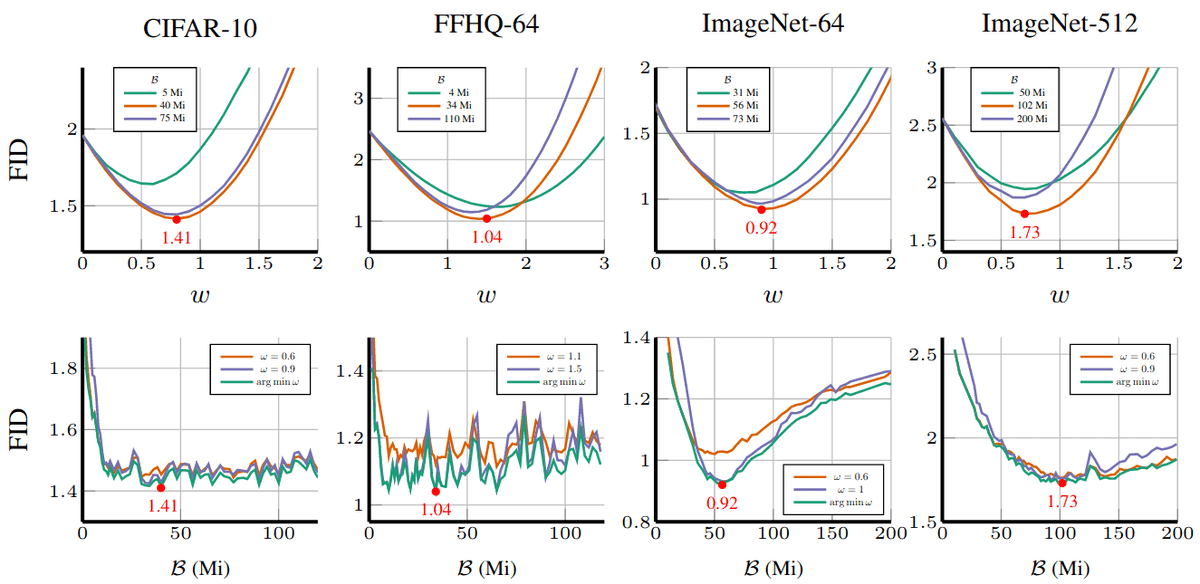
Top row: FID between the SIMS Algorithm and the real data distribution as a function of the guidance scale w at three different checkpoints of the training budget B as measured by the number of million-images-seen (Mi) during re-training of the auxiliary/impaired model. Bottom row: FID of the SIMS model as a function of training budget for three different values of the guidance scale w. Source
The above plot shows the impact of the training budget as measured by the number of samples seen during re-training and using different guidance strengths.
Smoothed Energy Guidance: Guiding Diffusion Models with Reduced Energy Curvature of Attention
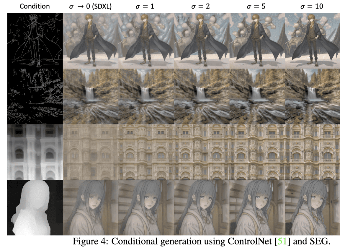
This is another approach to creating the negative model from the base model, called Smoothed Energy Guidance (SEG) . The authors manipulate a few self-attention blocks via blurring of the Stable Diffusion Unet. They also draw some connections between attention and Hopfield energy, as performing a self-attention operation is equivalent to taking a minimization gradient step in the energy landscape. The authors argue that Gaussian blurring on the attention weights modulates the underlying landscape to have less curvature, meaning it is smoother.
Blurring the attention weights means applying a localized Gaussian kernel with a specific standard deviation.
The kernel is slided across the image dimensions, and the mathematical operation is cross-correlation, or in deep learning terms, “convolution”. An important property of the Gaussian blurring is that the mean is preserved.
The 2D Gaussian filter is a set of weights of size K times K that uses a 2D Gaussian function to assign weights to neighboring pixels. The mean and variance are defined based on the pixel’s location, not their intensity. To the best of my knowledge, they fix the guidance scale and kernel size and only vary the sigma (standard deviation). Based on the open-source code, the kernel is computed as:
import math
kernel_size = math.ceil(6 * sigma) + 1 - math.ceil(6 * sigma) % 2
The advantages of SEG are that:
-
It is a tuning- and condition-free method
-
It can be interpreted as the “curvature of the underlying energy.”
-
Only the standard deviation (sigma) needs to be tuned.
However, a veiled limitation is that you must pick specific attention layers to apply smoothing, similar to previous methods (SAG and PAG).
Source
Conclusion
Overall, no single out-of-the-box method replaces the vanilla CFG, and more research is needed. This article briefly discussed ways to perform sampling with diffusion models in a CFG-like fashion. For more in-depth material, check out Coursera’s course on image generation or the new book from Manning Publications on Generative AI with PyTorch. If you feel like you‘ve learned something useful, share this blog post on social media or donate to help us reach a broader audience.
Citation
@article{adaloglou2024cfg,
title = "An overview of classifier-free guidance for diffusion models",
author = "Adaloglou, Nikolas, Kaiser, Tim",
journal = "theaisummer.com",
year = "2024",
url = "https://theaisummer.com/classifier-free-guidance"}
Disclaimer
Figures and tables shown in this work are provided based on arXiv preprints or published versions when available, with appropriate attribution to the respective works. Where the original works are available under a Creative Commons Attribution (CC BY 4.0) license, the reuse of figures and tables is explicitly permitted with proper attribution. For works without explicit licensing information, permissions have been requested from the authors, and any use falls under fair use consideration, aiming to support academic review and educational purposes. The use of any third-party materials is consistent with scholarly standards of proper citation and acknowledgment of sources.
References
* Disclosure: Please note that some of the links above might be affiliate links, and at no additional cost to you, we will earn a commission if you decide to make a purchase after clicking through.

